Chapter 13 of “Managerial Accounting: An Introduction to Concepts, Methods, and Uses” focuses on the allocation of costs to various responsibility centers within an organization. A responsibility center is a part of an organization whose manager is responsible for a particular set of activities. Proper cost allocation is crucial for accurate performance evaluation, budgeting, and decision-making.

Key Topics in Chapter 13

1. Understanding Responsibility Centers:

• Responsibility centers are segments within an organization, classified based on the level of responsibility managers have over costs, revenues, or investment in assets. The main types are:
  • Cost Centers: Responsible only for controlling costs (e.g., a manufacturing department).
  • Revenue Centers: Responsible for generating revenue (e.g., a sales department).
  • Profit Centers: Responsible for both revenues and costs, hence profitability (e.g., a product line).
  • Investment Centers: Responsible for revenues, costs, and the investment in assets used to generate profits (e.g., a division of a company).

1. Principles of Cost Allocation:

• The process of cost allocation involves assigning indirect costs (overhead) to different responsibility centers. The primary principles of cost allocation include:
  • Causality: Costs should be allocated based on the cause-and-effect relationship. This principle ensures that costs are assigned to centers based on their consumption of resources.
  • Benefits Received: Costs should be allocated to the centers that receive the benefits of the expenses.
  • Fairness and Equity: Cost allocation should be perceived as fair by all responsibility centers. This can be more subjective and depends on organizational culture.
  • Ability to Bear: Costs can be allocated based on the ability of a responsibility center to bear them, which often relates to the center’s size or profitability.

1. Methods of Cost Allocation:

• Direct Allocation Method: Allocates costs directly to the responsibility centers that incur them, without allocating any support department costs to other support departments.
• Step-Down Allocation Method: Allocates costs to both operating and support departments in a step-by-step manner, where some support department costs are allocated to other support departments.
• Reciprocal Allocation Method: Recognizes the mutual services provided among all support departments and allocates costs accordingly. This method is the most accurate but also the most complex.

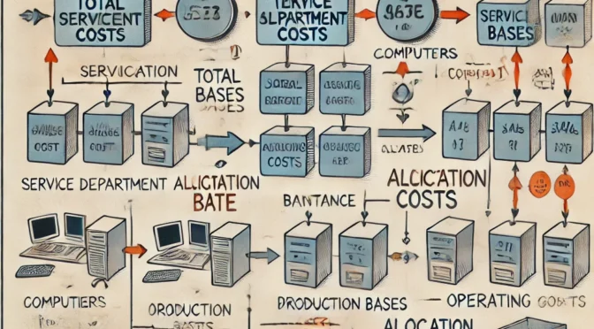
1. Allocating Service Department Costs:

• Service departments (e.g., IT, HR) provide services to other parts of the organization. The costs of these departments need to be allocated to the operating departments to determine the total cost of providing goods or services.
• The chapter discusses various methods for allocating service department costs, such as using direct labor hours, machine hours, or square footage as allocation bases.

1. Activity-Based Costing (ABC) for Cost Allocation:

• Activity-Based Costing is a more refined approach that assigns costs based on activities that drive costs. It involves identifying activities, assigning costs to these activities, and then allocating costs to products or services based on their consumption of those activities.

Math Problem and Solution from Chapter 13

To illustrate the Direct Allocation Method of allocating service department costs, consider the following problem:

Problem:
XYZ Corporation has two service departments, IT and Maintenance, and two operating departments, Production and Sales. The costs for IT and Maintenance are $100,000 and $50,000, respectively. The allocation bases are:

• IT costs are allocated based on the number of computers: Production has 60 computers, Sales has 40 computers.
• Maintenance costs are allocated based on square footage: Production occupies 2,000 square feet, Sales occupies 1,000 square feet.

Allocate the service department costs to the operating departments using the Direct Allocation Method.

Solution:

1. Calculate the Allocation Rate for IT Costs: The allocation rate for IT costs is calculated based on the number of computers. $$
   \text{IT Allocation Rate per Computer} = \frac{\text{Total IT Costs}}{\text{Total Number of Computers}}
   $$ Total number of computers = 60 (Production) + 40 (Sales) = 100 $$
   \text{IT Allocation Rate per Computer} = \frac{100,000}{100} = 1,000
   $$
2. Allocate IT Costs to Production and Sales:

• Production: $$
  \text{IT Costs for Production} = 60 \times 1,000 = 60,000
  $$
• Sales: $$
  \text{IT Costs for Sales} = 40 \times 1,000 = 40,000
  $$

1. Calculate the Allocation Rate for Maintenance Costs: The allocation rate for Maintenance costs is calculated based on square footage. $$
   \text{Maintenance Allocation Rate per Square Foot} = \frac{\text{Total Maintenance Costs}}{\text{Total Square Footage}}
   $$ Total square footage = 2,000 (Production) + 1,000 (Sales) = 3,000 $$
   \text{Maintenance Allocation Rate per Square Foot} = \frac{50,000}{3,000} = 16.67
   $$
2. Allocate Maintenance Costs to Production and Sales:

• Production: $$
  \text{Maintenance Costs for Production} = 2,000 \times 16.67 = 33,340
  $$
• Sales: $$
  \text{Maintenance Costs for Sales} = 1,000 \times 16.67 = 16,670
  $$

1. Total Allocated Costs:

• Production: IT ($60,000) + Maintenance ($33,340) = $93,340
• Sales: IT ($40,000) + Maintenance ($16,670) = $56,670

Conclusion

Chapter 13 emphasizes the importance of proper cost allocation in accurately measuring the performance of responsibility centers. By using methods such as the Direct Allocation Method, Step-Down Method, and Reciprocal Method, organizations can ensure that costs are fairly and accurately assigned to the appropriate departments. This enables better decision-making, budgeting, and performance evaluation, ultimately leading to more efficient and effective management of resources.

Chapter 12 of “Managerial Accounting: An Introduction to Concepts, Methods, and Uses” addresses the role of incentives in managerial accounting and how they influence managerial behavior and decision-making. Properly designed incentive systems are crucial for aligning the goals of individual managers with the overall objectives of the organization.

Key Topics in Chapter 12

1. The Role of Incentives in Organizations:

• Incentives are mechanisms used to motivate managers and employees to achieve organizational goals. These can be in the form of financial rewards, such as bonuses, stock options, or non-financial incentives like recognition and career advancement opportunities.
• A well-designed incentive system encourages managers to make decisions that are in the best interest of the company, aligning their actions with the company’s strategic objectives.

1. Types of Incentive Plans:

• Financial Incentives: Include bonuses, profit-sharing, stock options, and performance-based pay. These incentives are directly tied to financial performance metrics like net income, revenue growth, or cost savings.
• Non-Financial Incentives: Include recognition, promotions, professional development opportunities, and a positive work environment. These incentives focus on intrinsic motivation rather than purely financial rewards.

1. Linking Incentives to Performance Measures:

• Performance measures used to calculate incentives must be aligned with the organization’s goals and strategies. These measures can include financial metrics (such as ROI, residual income, and EVA) or non-financial metrics (such as customer satisfaction, employee turnover, and innovation rates).
• The choice of performance measures should reflect the aspects of performance that managers can control. For example, a sales manager might be evaluated on sales volume and customer satisfaction, while a production manager might be evaluated on cost control and production efficiency.

1. Challenges in Designing Effective Incentive Systems:

• Goal Congruence: Ensuring that the actions incentivized align with the overall goals of the organization. Poorly designed incentives may lead to behavior that benefits individual managers but is detrimental to the organization.
• Measurement Issues: Performance measures must be accurate, reliable, and timely. Inaccurate measures can lead to unfair rewards or penalties, reducing the effectiveness of the incentive system.
• Risk and Uncertainty: Managers should not be penalized or excessively rewarded for outcomes outside their control. Incentive systems need to account for the inherent risks and uncertainties in different business environments.

1. Behavioral Aspects of Incentives:

• Incentive systems can influence not only what managers do but also how they do it. For instance, a focus on short-term profits might discourage investment in long-term growth or innovation.
• The chapter also discusses the potential for dysfunctional behavior, such as manipulation of performance measures or focusing only on incentivized tasks while neglecting other important but non-incentivized activities.

Math Problem and Solution from Chapter 12

To illustrate the impact of incentives on managerial decision-making, consider the following problem involving a bonus plan based on ROI.

Problem:
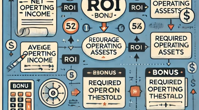
ABC Corporation offers its division managers a bonus of 5% of the division’s net operating income if the division’s ROI exceeds 15%. Division X has average operating assets of $1,200,000 and achieved a net operating income of $210,000 this year. Calculate the division’s ROI and determine if the manager is eligible for the bonus. If eligible, calculate the bonus amount.

Solution:

1. Calculate the Return on Investment (ROI): ROI is calculated to determine if the division’s performance meets the threshold for the bonus. $$
   \text{ROI} = \frac{\text{Net Operating Income}}{\text{Average Operating Assets}}
   $$ Substituting the values: $$
   \text{ROI} = \frac{210,000}{1,200,000} = 0.175 \, \text{or} \, 17.5\%
   $$ Since the ROI of 17.5% exceeds the required threshold of 15%, the manager is eligible for the bonus.
2. Calculate the Bonus Amount: The bonus is 5% of the net operating income since the division achieved an ROI above the threshold. $$
   \text{Bonus} = \text{Net Operating Income} \times \text{Bonus Percentage}
   $$ Substituting the values: $$
   \text{Bonus} = 210,000 \times 0.05 = 10,500
   $$
3. Interpretation of Results: The manager of Division X is eligible for a bonus of $10,500, given that the division’s ROI of 17.5% exceeds the 15% threshold set by the company. This illustrates how incentive systems can be designed to motivate managers to achieve specific financial targets, thereby aligning their efforts with the organization’s goals.

Conclusion

Chapter 12 highlights the critical role of incentive systems in influencing managerial behavior and aligning individual efforts with organizational objectives. Effective incentive plans must be well-designed to ensure goal congruence, fairness, and motivation, while avoiding unintended consequences that may lead to dysfunctional behavior. By linking incentives to appropriate performance measures, organizations can foster a culture of performance and continuous improvement.

Chapter 11 of “Managerial Accounting: An Introduction to Concepts, Methods, and Uses” focuses on evaluating the performance of investment centers within an organization. An investment center is a segment of an organization where the manager is responsible not only for generating revenue and controlling costs but also for the efficient use of the assets invested in the segment.

Key Topics in Chapter 11

1. Definition of Investment Centers:

• An Investment Center is a business unit or division whose manager is responsible for its profits and the return on the investment made in it. This setup allows for evaluating a manager’s performance based on both profitability and the efficient use of assets.

1. Performance Measures for Investment Centers:

• Return on Investment (ROI): A widely used measure of performance, ROI indicates how effectively a division uses its assets to generate profits.
• Residual Income (RI): Measures the absolute amount of profit generated above a required return on invested capital. It provides a dollar amount rather than a percentage.
• Economic Value Added (EVA): A performance measure that adjusts for accounting distortions to better reflect economic profit, considering the cost of capital.

1. Calculating ROI:

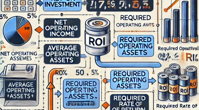
• ROI is calculated as: $$
  \text{ROI} = \frac{\text{Net Operating Income}}{\text{Average Operating Assets}}
  $$
• This formula measures the profitability relative to the assets employed. Higher ROI indicates better use of assets to generate earnings.

1. Advantages and Disadvantages of ROI:

• Advantages: ROI is simple to calculate and widely understood. It facilitates comparisons across divisions and is useful for benchmarking.
• Disadvantages: ROI can incentivize managers to avoid investments that may benefit the company but lower their division’s ROI. It can also discourage the replacement of fully depreciated but inefficient assets.

1. Calculating Residual Income (RI):

• RI is calculated as: $$
  \text{RI} = \text{Net Operating Income} – (\text{Average Operating Assets} \times \text{Required Rate of Return})
  $$
• RI considers both the cost of capital and the profit generated, making it a better measure for aligning managerial decisions with the overall company’s goals.

1. Economic Value Added (EVA):

• EVA is similar to RI but adjusts for certain accounting practices to provide a clearer picture of economic profit. It is calculated as: $$
  \text{EVA} = \text{Net Operating Profit After Taxes (NOPAT)} – (\text{Invested Capital} \times \text{Weighted Average Cost of Capital (WACC)})
  $$

Math Problem and Solution from Chapter 11

Problem:
Division B of ABC Corporation has average operating assets of $800,000 and generates a net operating income of $160,000. The company’s required rate of return is 12%. Calculate the Return on Investment (ROI) and Residual Income (RI) for Division B.

Solution:

1. Calculate the Return on Investment (ROI): ROI measures the efficiency of the investment in generating operating income. $$
   \text{ROI} = \frac{\text{Net Operating Income}}{\text{Average Operating Assets}}
   $$ Substituting the values: $$
   \text{ROI} = \frac{160,000}{800,000} = 0.20 \, \text{or} \, 20\%
   $$
2. Calculate the Residual Income (RI): RI measures the absolute amount of income generated above the required return on operating assets. $$
   \text{RI} = \text{Net Operating Income} – (\text{Average Operating Assets} \times \text{Required Rate of Return})
   $$ Substituting the values: $$
   \text{RI} = 160,000 – (800,000 \times 0.12)
   $$ $$
   \text{RI} = 160,000 – 96,000 = 64,000
   $$
3. Interpretation of Results:

• ROI: The division’s ROI is 20%, indicating that for every dollar invested in assets, the division generates $0.20 in operating income.
• RI: The division’s RI is $64,000, indicating that it generated $64,000 more than the required return on its operating assets. This means Division B is creating value above the minimum acceptable rate of return.

Conclusion

Chapter 11 highlights the importance of using appropriate performance measures to evaluate the effectiveness of investment center managers. By using ROI, RI, and EVA, companies can ensure that managers are making decisions that align with overall corporate goals, effectively utilizing assets, and creating shareholder value. Each measure has its strengths and weaknesses, and the choice of metric depends on the company’s strategic objectives and the specific context of each division.

Chapter 10 of “Managerial Accounting: An Introduction to Concepts, Methods, and Uses” focuses on identifying relevant costs for decision-making. Relevant costs are crucial in short-term business decisions, as they directly affect the financial outcomes of various strategic choices.

Key Topics in Chapter 10

1. Understanding Relevant Costs:

• Relevant costs are costs that will change as a result of a decision. They are future costs that differ between alternatives. Only these costs should be considered when making decisions.
• Irrelevant costs are costs that do not change between alternatives or are sunk costs (costs already incurred and cannot be recovered).

1. Types of Relevant Costs:

• Avoidable Costs: Costs that can be eliminated if a particular decision is made.
• Incremental Costs: Additional costs that occur if a specific action is taken.
• Opportunity Costs: The benefits foregone by choosing one alternative over another.

1. Common Decision-Making Scenarios:

• Make or Buy Decisions: Involves deciding whether to produce a component in-house or purchase it from an external supplier.
• Special Order Decisions: Determining whether to accept an order at a price lower than the normal selling price, typically to utilize excess capacity.
• Product Line Decisions: Deciding whether to add or drop a product line or business segment based on profitability.
• Sell or Process Further Decisions: Determining whether to sell a product as is or process it further to enhance its value.
• Resource Allocation Decisions: Choosing how to allocate limited resources among different products or services to maximize profitability.

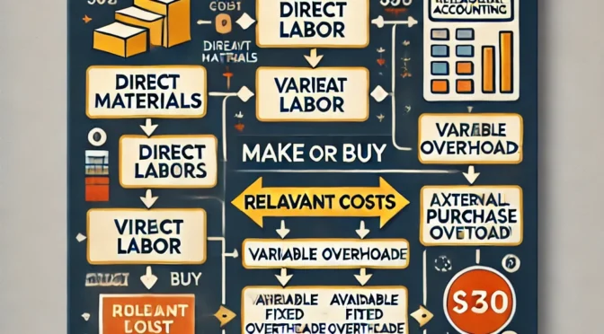
1. Make or Buy Analysis:

• This analysis involves comparing the relevant costs of making a product internally versus buying it from an external supplier. Relevant costs typically include direct materials, direct labor, variable overhead, and any avoidable fixed costs.

Math Problem and Solution from Chapter 10

To illustrate Make or Buy Decisions, consider the following problem:

Problem:
XYZ Company is currently producing a component internally at the following costs for 10,000 units per year:

• Direct Materials: $2 per unit
• Direct Labor: $4 per unit
• Variable Overhead: $1 per unit
• Fixed Overhead: $3 per unit (of which $2 per unit is avoidable if production is outsourced)

An external supplier offers to provide the component at $8 per unit. Should XYZ Company continue to make the component or buy it from the external supplier?

Solution:

1. Calculate the Relevant Costs of Making the Component: Relevant costs include all variable costs and avoidable fixed costs:

• Direct Materials Cost: $$
  \text{Direct Materials Cost} = 2 \times 10,000 = 20,000
  $$
• Direct Labor Cost: $$
  \text{Direct Labor Cost} = 4 \times 10,000 = 40,000
  $$
• Variable Overhead Cost: $$
  \text{Variable Overhead Cost} = 1 \times 10,000 = 10,000
  $$
• Avoidable Fixed Overhead Cost: $$
  \text{Avoidable Fixed Overhead Cost} = 2 \times 10,000 = 20,000
  $$ Total Relevant Costs of Making: $$
  \text{Total Relevant Cost (Make)} = 20,000 + 40,000 + 10,000 + 20,000 = 90,000
  $$

1. Calculate the Cost of Buying the Component: If the company buys the component, the cost will be: $$
   \text{Total Cost (Buy)} = 8 \times 10,000 = 80,000
   $$
2. Compare the Costs:

• Cost of Making: $90,000
• Cost of Buying: $80,000 Since the cost of buying ($80,000) is less than the cost of making ($90,000), XYZ Company should buy the component from the external supplier.

1. Opportunity Cost Consideration: If there are no opportunity costs associated with using the company’s facilities for another purpose, the decision to buy is clear. However, if the facilities can be used for a more profitable purpose, that opportunity cost should be included in the decision analysis.

Conclusion

Chapter 10 emphasizes the importance of understanding relevant costs when making managerial decisions. By focusing only on costs that will change as a result of a decision, managers can make more informed choices that align with the company’s strategic objectives. Whether it’s deciding to make or buy a product, accept a special order, or allocate resources, identifying relevant costs is key to maximizing profitability and operational efficiency.

Chapter 9 of “Managerial Accounting: An Introduction to Concepts, Methods, and Uses” focuses on the concepts of decentralization and performance evaluation within organizations. Decentralization refers to the distribution of decision-making authority to lower levels within the organization, while performance evaluation involves assessing the effectiveness of these decisions and the managers who make them.

Key Topics in Chapter 9

1. Decentralization in Organizations:

• Decentralization allows decision-making authority to be distributed among various levels of management, rather than being concentrated at the top. It empowers managers to make decisions that are closer to their specific areas of responsibility.
• Benefits of decentralization include faster decision-making, increased motivation among managers, and better use of local knowledge.
• Potential drawbacks include a lack of goal congruence, where individual managers’ goals may not align with the organization’s overall objectives, and the possibility of inefficiencies due to duplicated efforts.

1. Responsibility Centers:

• A responsibility center is a part of an organization whose manager is accountable for specific activities. Responsibility centers can be classified into four types:
  • Cost Centers: Managers are responsible for controlling costs but not for generating revenue (e.g., a manufacturing department).
  • Revenue Centers: Managers are responsible for generating revenue but not for controlling costs (e.g., a sales department).
  • Profit Centers: Managers are responsible for both generating revenue and controlling costs (e.g., a product line).
  • Investment Centers: Managers are responsible for revenues, costs, and investments in assets (e.g., a division of a company).

1. Performance Evaluation Methods:

• Various methods are used to evaluate the performance of responsibility centers, including:
  • Variance Analysis: Comparing actual results with budgeted or standard costs and revenues to determine variances.
  • Return on Investment (ROI): A measure of profitability and efficiency, calculated as net operating income divided by average operating assets.
  • Residual Income (RI): A measure that considers both operating income and the cost of capital. It is calculated as net operating income minus a charge for the cost of capital employed in the center.
  • Economic Value Added (EVA): Similar to residual income, but with adjustments for accounting practices to better reflect economic performance.

1. Transfer Pricing:

• Transfer pricing refers to the price charged for goods or services transferred between divisions within the same organization. It affects the profitability of both the selling and buying divisions.
• Common methods for setting transfer prices include market-based prices, cost-based prices, and negotiated prices. The choice of transfer pricing method can impact divisional performance evaluations and overall organizational effectiveness.

Math Problem and Solution from Chapter 9

To illustrate Return on Investment (ROI) and Residual Income (RI), consider the following problem:

Problem:
Division A of XYZ Corporation has an average operating asset base of $500,000. The division’s net operating income for the year is $100,000. XYZ Corporation requires a minimum return on investment of 15%. Calculate the Return on Investment (ROI) and Residual Income (RI) for Division A.

Solution:

1. Calculate the Return on Investment (ROI): ROI is a measure of the profitability of a division relative to its operating assets. $$
   \text{Return on Investment (ROI)} = \frac{\text{Net Operating Income}}{\text{Average Operating Assets}}
   $$ Substituting the values: $$
   \text{ROI} = \frac{100,000}{500,000} = 0.20 \, \text{or} \, 20\%
   $$
2. Calculate the Residual Income (RI): Residual Income measures the net operating income above the minimum required return on average operating assets. $$
   \text{Residual Income (RI)} = \text{Net Operating Income} – (\text{Minimum Required Return} \times \text{Average Operating Assets})
   $$ Substituting the values: $$
   \text{RI} = 100,000 – (0.15 \times 500,000)
   $$ $$
   \text{RI} = 100,000 – 75,000 = 25,000
   $$
3. Interpretation of Results:

• ROI: The division’s ROI is 20%, which is above the required minimum of 15%, indicating efficient use of assets.
• RI: The division’s RI is $25,000, indicating that it generated $25,000 above the minimum required return on its operating assets.

Conclusion

Chapter 9 discusses the importance of decentralization and effective performance evaluation methods to ensure that managers make decisions aligned with the organization’s goals. Tools such as ROI, RI, and EVA provide insights into the performance of different responsibility centers, helping management make informed decisions about resource allocation and strategic direction. Properly setting transfer prices also ensures fairness and encourages optimal decision-making across divisions.

Chapter 8 of “Managerial Accounting: An Introduction to Concepts, Methods, and Uses” focuses on Standard Costing and Variance Analysis, two crucial tools in managerial accounting. These concepts help managers control costs, evaluate performance, and make informed decisions by comparing actual costs to pre-established standards.

Key Topics in Chapter 8

1. Standard Costing:

• Standard Costing involves setting predetermined costs for products or services, which are used as benchmarks to measure actual performance. These standard costs are based on expected levels of efficiency and input prices.
• The components of standard costs typically include Direct Materials, Direct Labor, and Manufacturing Overhead (both variable and fixed).

1. Types of Standards:

• Ideal Standards: Based on perfect operating conditions with no allowances for waste or inefficiency. These are rarely achieved in practice and can be demotivating if used for performance evaluation.
• Practical (Attainable) Standards: Based on efficient operating conditions with normal allowances for waste, spoilage, and downtime. These are more realistic and motivating for employees.

1. Variance Analysis:

• Variance analysis is the process of comparing actual costs to standard costs to determine the reasons for variances. It helps in identifying areas where performance did not meet expectations and provides insights into where corrective actions are needed.
• Favorable Variance: Occurs when actual costs are lower than standard costs, indicating better-than-expected performance.
• Unfavorable Variance: Occurs when actual costs are higher than standard costs, indicating poorer-than-expected performance.

1. Types of Variances:

• Direct Material Variances:
  • Material Price Variance: Measures the difference between the actual price paid for materials and the standard price.
  • Material Quantity Variance: Measures the difference between the actual quantity of materials used and the standard quantity allowed for actual production.
• Direct Labor Variances:
  • Labor Rate Variance: Measures the difference between the actual hourly wage rate paid and the standard rate.
  • Labor Efficiency Variance: Measures the difference between the actual labor hours used and the standard hours allowed for actual production.
• Overhead Variances:
  • Variable Overhead Variance: Consists of the Spending Variance (difference between actual variable overhead costs and standard variable overhead costs based on actual hours) and Efficiency Variance (difference between the actual hours worked and standard hours allowed).
  • Fixed Overhead Variance: Consists of the Spending Variance and Volume Variance.

Math Problem and Solution from Chapter 8

To illustrate Standard Costing and Variance Analysis, consider the following problem:

Problem:
XYZ Company sets a standard cost of $5 per unit for direct materials. The standard quantity allowed for actual production is 4,000 units. The company purchased and used 4,200 units of material at an actual cost of $4.80 per unit. Calculate the Material Price Variance and Material Quantity Variance.

Solution:

1. Calculate the Material Price Variance (MPV): The Material Price Variance measures the difference between the actual price paid for materials and the standard price, multiplied by the actual quantity purchased. $$
   \text{Material Price Variance (MPV)} = (\text{Actual Price} – \text{Standard Price}) \times \text{Actual Quantity}
   $$ Substituting the values: $$
   \text{MPV} = (4.80 – 5.00) \times 4,200 = -0.20 \times 4,200 = -840
   $$ The negative variance indicates a favorable variance because the actual price was lower than the standard price.
2. Calculate the Material Quantity Variance (MQV): The Material Quantity Variance measures the difference between the actual quantity of materials used and the standard quantity allowed for actual production, multiplied by the standard price. $$
   \text{Material Quantity Variance (MQV)} = (\text{Actual Quantity} – \text{Standard Quantity}) \times \text{Standard Price}
   $$ The standard quantity allowed for actual production (4,000 units of material) is compared to the actual quantity used (4,200 units): $$
   \text{MQV} = (4,200 – 4,000) \times 5.00 = 200 \times 5.00 = 1,000
   $$ The positive variance indicates an unfavorable variance because more materials were used than allowed.
3. Interpretation of Variances:

• Material Price Variance (MPV): The variance is favorable ($-840) because the company paid less per unit for materials than the standard cost.
• Material Quantity Variance (MQV): The variance is unfavorable ($1,000) because more materials were used than the standard quantity allowed for actual production.

Conclusion

Chapter 8 emphasizes the importance of standard costing and variance analysis in cost control and performance evaluation. By setting standard costs and analyzing variances, managers can identify areas where efficiency can be improved, costs can be controlled, and resources can be better utilized. Understanding the reasons behind variances allows managers to take corrective actions and make informed decisions to enhance organizational performance.

Chapter 7 of “Managerial Accounting: An Introduction to Concepts, Methods, and Uses” focuses on the role of budgeting in managerial planning and control. Budgeting is a crucial tool for management to set financial targets, allocate resources, and monitor performance against those targets.

Key Topics in Chapter 7

1. Purpose of Budgeting:

• Budgeting serves multiple purposes, including planning, coordination, communication, and control. It helps managers set goals, anticipate future challenges, and align the activities of different departments.
• Budgets provide a framework for evaluating performance by comparing actual results against budgeted figures.

1. Types of Budgets:

• Master Budget: A comprehensive budget that consolidates all individual departmental budgets. It includes the operating budget, capital expenditure budget, and financial budget (cash budget, budgeted income statement, and budgeted balance sheet).
• Operating Budgets: These budgets relate to the day-to-day operations of the business and include sales, production, direct materials, direct labor, manufacturing overhead, and selling and administrative expenses budgets.
• Financial Budgets: These focus on the financial aspects of the business, such as the cash budget, budgeted income statement, and budgeted balance sheet.

1. The Budgeting Process:

• Sales Budget: The starting point for the budgeting process. It forecasts the expected sales in units and dollars and forms the basis for other budgets.
• Production Budget: Based on the sales budget, it determines the number of units that need to be produced to meet sales and inventory requirements.
• Direct Materials, Direct Labor, and Overhead Budgets: These budgets estimate the costs associated with the production process, including materials required, labor hours needed, and overhead expenses.

1. Flexible Budgets:

• A flexible budget adjusts for different levels of activity. It is more useful than a static budget when comparing actual performance because it reflects what costs should have been at the actual level of activity.
• Flexible budgets help in variance analysis by providing a more accurate comparison of actual costs against budgeted costs at the actual activity level.

1. Variance Analysis:

• Variance analysis is the process of comparing actual results to budgeted figures and analyzing the reasons for any differences. It helps in identifying areas that require management’s attention and corrective actions.
• Common variances include sales volume variance, sales price variance, direct materials variance, direct labor variance, and overhead variance.

Math Problem and Solution from Chapter 7

To illustrate the Flexible Budget and Variance Analysis, consider the following problem:

Problem:
XYZ Manufacturing prepared a static budget for producing 5,000 units, with the following cost estimates:

• Direct materials: $10 per unit
• Direct labor: $15 per unit
• Variable overhead: $5 per unit
• Fixed overhead: $20,000

However, the actual production was 6,000 units. Prepare a flexible budget and calculate the variances for each cost category.

Solution:

1. Prepare the Flexible Budget: The flexible budget adjusts the costs based on the actual level of activity (6,000 units). Flexible Budget Calculation:

• Direct Materials Cost: $$
  \text{Direct Materials Cost} = \text{Direct Materials per Unit} \times \text{Actual Units Produced}
  $$ $$
  \text{Direct Materials Cost} = 10 \times 6,000 = 60,000
  $$
• Direct Labor Cost: $$
  \text{Direct Labor Cost} = \text{Direct Labor per Unit} \times \text{Actual Units Produced}
  $$ $$
  \text{Direct Labor Cost} = 15 \times 6,000 = 90,000
  $$
• Variable Overhead Cost: $$
  \text{Variable Overhead Cost} = \text{Variable Overhead per Unit} \times \text{Actual Units Produced}
  $$ $$
  \text{Variable Overhead Cost} = 5 \times 6,000 = 30,000
  $$
• Fixed Overhead Cost: Fixed costs remain unchanged regardless of the level of activity within the relevant range. $$
  \text{Fixed Overhead Cost} = 20,000
  $$ Total Flexible Budget Cost: $$
  \text{Total Cost} = \text{Direct Materials Cost} + \text{Direct Labor Cost} + \text{Variable Overhead Cost} + \text{Fixed Overhead Cost}
  $$ $$
  \text{Total Cost} = 60,000 + 90,000 + 30,000 + 20,000 = 200,000
  $$

1. Calculate Variances: If the actual costs were:

• Direct materials: $58,000
• Direct labor: $93,000
• Variable overhead: $33,000
• Fixed overhead: $21,000 Then, the variances are calculated as:
• Direct Materials Variance: $$
  \text{Direct Materials Variance} = \text{Actual Cost} – \text{Flexible Budget Cost}
  $$ $$
  \text{Direct Materials Variance} = 58,000 – 60,000 = -2,000 \, (\text{Favorable})
  $$
• Direct Labor Variance: $$
  \text{Direct Labor Variance} = 93,000 – 90,000 = 3,000 \, (\text{Unfavorable})
  $$
• Variable Overhead Variance: $$
  \text{Variable Overhead Variance} = 33,000 – 30,000 = 3,000 \, (\text{Unfavorable})
  $$
• Fixed Overhead Variance: $$
  \text{Fixed Overhead Variance} = 21,000 – 20,000 = 1,000 \, (\text{Unfavorable})
  $$

Conclusion

Chapter 7 emphasizes the importance of budgeting in managerial planning and control. Budgets provide a financial framework for setting goals, allocating resources, and measuring performance. Flexible budgets and variance analysis enable managers to adjust for actual activity levels and identify areas needing improvement, ensuring that the organization remains on track to achieve its financial objectives.