Key Concepts and Detailed Discussion:
1. Introduction to Queuing Theory:
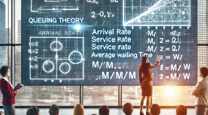
Queuing theory, also known as the study of waiting lines, is one of the oldest and most widely used techniques in quantitative analysis. It provides mathematical models for analyzing various types of queuing systems encountered in real-life situations, such as customers waiting in line at a bank, vehicles waiting at a traffic light, or data packets waiting to be processed in a network.
2. Components of a Queuing System:
A queuing system is characterized by three main components:
- Arrival Process: Describes how customers or entities arrive at the queue. It includes arrival rate, distribution, and the nature of the arrivals (e.g., single or batch).
- Service Process: Involves the manner in which customers are served once they reach the service facility. It includes service rate, service time distribution, and number of service channels.
- Queue Discipline: Refers to the rules determining the order in which customers are served, such as first-come-first-served (FCFS), last-come-first-served (LCFS), or priority-based.
3. Key Queuing Models:
Several standard queuing models are discussed, each suited to different types of queuing systems. The most common models include:
3.1. Single-Channel Queuing Model (M/M/1):
The M/M/1 model is a basic single-server queuing system where arrivals follow a Poisson distribution and service times follow an exponential distribution.
- Assumptions of the M/M/1 Model:
- Arrivals are Poisson-distributed with mean arrival rate (\lambda).
- Service times are exponentially distributed with mean service rate (\mu).
- There is a single server.
- The queue has an infinite capacity, and customers are served on a first-come, first-served basis.
- Queuing Equations for the M/M/1 Model:
The following are key performance measures for the M/M/1 model:
- Average number of customers in the system (L):
$$
L = \frac{\lambda}{\mu – \lambda}
$$ - Average time a customer spends in the system (W):
$$
W = \frac{1}{\mu – \lambda}
$$ - Average number of customers in the queue (L_q):
$$
L_q = \frac{\lambda^2}{\mu(\mu – \lambda)}
$$ - Average time a customer spends waiting in the queue (W_q):
$$
W_q = \frac{\lambda}{\mu(\mu – \lambda)}
$$
3.2. Multi-Channel Queuing Model (M/M/m):
The M/M/m model extends the M/M/1 model to multiple servers (channels) but still assumes Poisson arrivals and exponential service times.
- Equations for the Multichannel Queuing Model:
- Probability that all servers are busy (P_0): $$
P_0 = \left[ \sum_{n=0}^{m-1} \frac{(\lambda/\mu)^n}{n!} + \frac{(\lambda/\mu)^m}{m! \left(1 – \frac{\lambda}{m\mu}\right)} \right]^{-1}
$$ - Average number of customers in the system (L): $$
L = \frac{\lambda \mu (\lambda/\mu)^m}{(m-1)!(m\mu – \lambda)^2} P_0 + \frac{\lambda}{\mu}
$$
3.3. Constant Service Time Model (M/D/1):
The M/D/1 model assumes Poisson arrivals and deterministic (constant) service times.
- Key Equations for M/D/1:
- Average number of customers in the system (L): $$
L = \frac{\lambda^2}{2\mu(\mu – \lambda)} + \frac{\lambda}{\mu}
$$ - Average time a customer spends in the system (W): $$
W = \frac{\lambda}{2\mu(\mu – \lambda)} + \frac{1}{\mu}
$$
3.4. Finite Population Model (M/M/1 with Finite Source):
This model is appropriate when the population size is limited, such as a fixed number of machines waiting for repair.
- Equations for the Finite Population Model:
The performance measures are adjusted to account for the limited source of arrivals.
4. Operating Characteristics and General Relationships:
Understanding the general operating characteristics, such as utilization factor ((\rho = \frac{\lambda}{m\mu})), helps managers evaluate and optimize service efficiency. Relationships between these characteristics provide insights into how changes in service rates or arrival rates impact the system.
5. Cost Considerations in Queuing Models:
The cost components in a queuing system typically include:
- Service Cost: The cost associated with providing service, including salaries and operational expenses.
- Waiting Cost: The cost associated with customer waiting time, which can be tangible (lost business) or intangible (customer dissatisfaction).
Managers aim to balance these costs to minimize the total cost of the queuing system.
6. Simulation of Queuing Models:
When analytical solutions are not feasible or practical, simulation methods can be used to model and analyze more complex queuing systems. Simulation allows for a more flexible analysis of various scenarios and configurations.
Summary:
Chapter 13 provides a comprehensive overview of waiting lines and queuing theory models, covering their structure, key characteristics, mathematical modeling, and applications in various service environments. By applying these models, businesses can optimize their operations to enhance customer satisfaction and reduce costs associated with waiting times.
